45 excel doughnut chart labels outside
How to Create Doughnut Excel Chart? - WallStreetMojo doughnut chart is a type of chart in excel whose function of visualization is just similar to pie charts, the categories represented in this chart are parts and together they represent the whole data in the chart, only the data which are in rows or columns only can be used in creating a doughnut chart in excel, however it is advised to use this … Doughnut Chart | Basic Charts | AnyChart Documentation A doughnut (or donut) chart is a pie chart with a "hole" - a blank circular area in the center. The chart is divided into parts that show the percentage each value contributes to a total. Like the regular pie chart, the doughnut chart is used with small sets of data to compare categories. It drives attention from the area taken by each part to ...
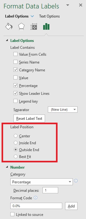
How to make data label position appear on the outside of chart for ... We have looked into your issue further and found that doughnet chart data labels cannot be positioned outside using Microsoft Excel. If something is not possible with Microsoft Excel, it will automatically be not possible with Aspose.Cells. I have also attached the screenshot highlighting my point for your reference. STL June 29, 2017, 6:29am #7
Excel doughnut chart labels outside
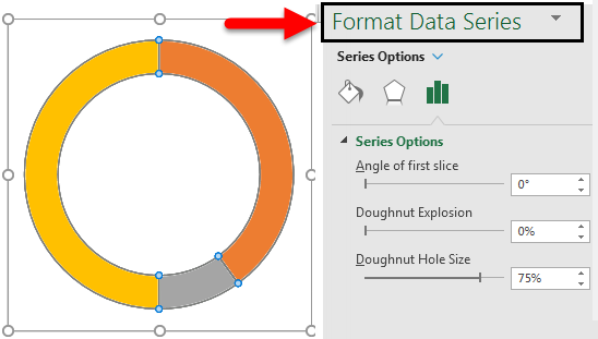
Labels for pie and doughnut charts - Support Center Format labels To format labels for pie and doughnut charts: 1 Select your chart or a single slice. Turn the slider on to Show Label. 2 Use the sliders to choose whether to include Name, Value, and Percent. 3 Use the Precision setting allows you to determine how many digits display for numeric values. 4 How to make doughnut chart with outside end labels? - Simple Excel VBA ... In the doughnut type charts Excel gives You no option to change the position of data label. The only setting is to have them inside the chart. exceldashboardschool.com › radial-bar-chartCreate Radial Bar Chart in Excel - Step by step Tutorial Jun 25, 2022 · Then, go to Ribbon and Insert tab, Chart, and Insert a Doughnut Chart. Step 5: Click on the inserted chart. Select the chart area. Right-click on the chart, and finally click on “select data”. A new popup window will be opened. Step 6: Click on the Switch Row/Column button. Step 7: Now, right-click on the doughnut and click on Format Data ...
Excel doughnut chart labels outside. › excel_charts › excel_chartsExcel Charts - Chart Elements - Tutorials Point You can change the location of the data labels within the chart, to make them more readable. Step 4 − Click the icon to see the options available for data labels. Step 5 − Point on each of the options to see how the data labels will be located on your chart. For example, point to data callout. The data labels are placed outside the pie ... Interactive Donut Chart - Beat Excel! Now select and copy the first gray area in Sheet 2 that includes blue donut part and paste it as a linked picture to cell B2 of Sheet 1. Click on this picture and type =Chart inside the formula bar. Do the same with the label but this time place it in the middle of the gray area in Sheet 1. While on Sheet 1, insert a donut chart as shown below. Fix label position in doughnut chart? - MrExcel Message Board Turn off data labels. Insert a Text box in to the middle of the donut, select the edge of the text box and in the formula bar hit = then select the cell that contains the progress figure. You can format this to however you want it, it will update and it won't move. Click to expand... Oh wow! I always thought text-boxes were just text-boxes. excel - Positioning labels on a donut-chart - Stack Overflow The option to place the labels outside the chart is not available on the doughnut chart options: like they do on a pie chart: However, you could perform a trick using a pie chart and a white circle to make it look like a doughnut by doing the following: Sub AddCircle () 'Get chart size and position: Dim CH01 As Chart: Set CH01 = ThisWorkbook ...
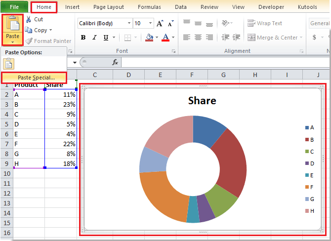
How to Create a Double Doughnut Chart in Excel - Statology Step 3: Add a layer to create a double doughnut chart. Right click on the doughnut chart and click Select Data. In the new window that pops up, click Add to add a new data series. For Series values, type in the range of values fpr Quarter 2 revenue: Click OK. Excel Doughnut chart with leader lines - teylyn Step 1 - doughnut chart with data labels Step 2 -Add the same data series as a pie chart Next, select the data again, categories and values. Copy the data, then click the chart and use the Paste Special command. Specify that the data is a new series and hit OK. You will see the new data series as an outer ring on the doughnut chart. How to create a creative multi-layer Doughnut Chart in Excel By default, all doughnut chart layers have a borderline. As this border line is only disrupting the look, you should remove it for all borders first. After that, select the outer layer of the second (also second biggest) data point and set the fill to No fill. For the third data point we apply the same technique to the two outer layers, and so on. Conditional formatting for donut chart | Think Outside The Slide Jon Acampora of Excel Campus has created two videos on creating a donut chart that has conditional formatting so that the segment that represents progress changes color based on the percentage value. The first video goes over the basic steps to create a donut chart. The second video extends this to add conditional formatting to the donut chart.
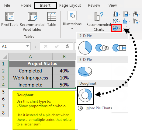
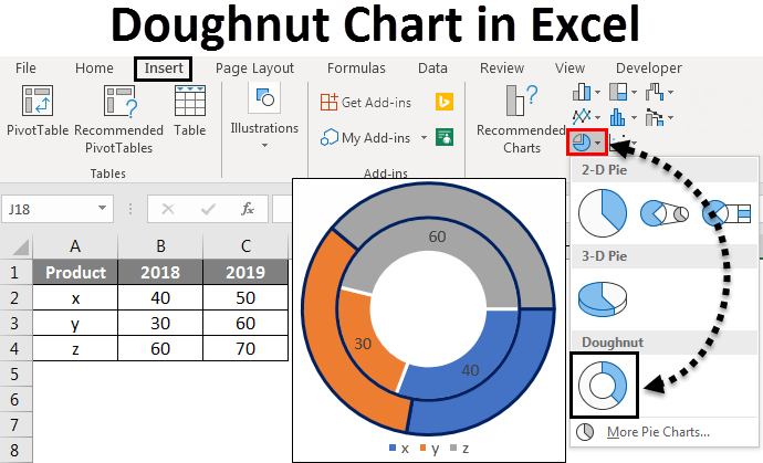
Excel charts: add title, customize chart axis, legend and data labels Click anywhere within your Excel chart, then click the Chart Elements button and check the Axis Titles box. If you want to display the title only for one axis, either horizontal or vertical, click the arrow next to Axis Titles and clear one of the boxes: Click the axis title box on the chart, and type the text. Using Pie Charts and Doughnut Charts in Excel To create one chart of this data, follow these steps: 1. Select the first data range (in this example, B5:C10 ). 2. On the Insert tab, in the Charts group, select the Pie and Doughnut button: In the Pie and Doughnut dropdown list, choose the Doughnut chart. 3. Right-click in the chart area and do one of the following: Under Chart Tools, on the ... › pie-chart-in-excelPie Chart in Excel | How to Create Pie Chart - EDUCBA Excel Pie Chart ( Table of Contents ) Pie Chart in Excel; How to Make Pie Chart in Excel? Pie Chart in Excel. Pie Chart in Excel is used for showing the completion or main contribution of different segments out of 100%. It is like each value represents the portion of the Slice from the total complete Pie. For Example, we have 4 values A, B, C ... › charts › progProgress Doughnut Chart with Conditional Formatting in Excel Go to the Insert tab and select Doughnut Chart from the Pie Chart drop-down menu. The doughnut chart will be inserted on the sheet. Step 3 - Format the Doughnut Chart Now we need to modify the formatting of the chart to highlight the progress bar. The default chart will look something like the following. Here are the steps to clean it up.
How to add leader lines to doughnut chart in Excel?
support.microsoft.com › en-us › officeAvailable chart types in Office - support.microsoft.com Doughnut chart Like a pie chart, a doughnut chart shows the relationship of parts to a whole. However, it can contain more than one data series. Each ring of the doughnut chart represents a data series. Displays data in rings, where each ring represents a data series. If percentages are displayed in data labels, each ring will total 100%.

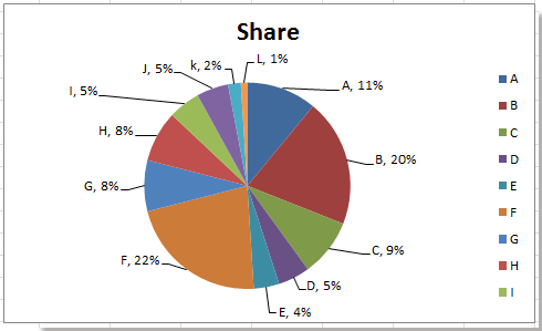
How to show percentages on three different charts in Excel - Excel Board
How to create doughnut chart in Excel? - ExtendOffice 1. Select the data range you need to be shown in the doughnut chart, and click Insert > Other Charts > Doughnut. See screenshot: In Excel 2013, click Insert > Insert Pie or Doughnut Chart > Doughnut. See screenshot: 2. Then a doughnut chart is inserted in your worksheet. Now you can right click at all series and select Add Data Labels from the ...

Add label to center of C# Excel Doughnut chart - Stack Overflow
Label position - outside of chart for Doughnut charts - VBA Solution ... The doughnut chart label options are not good... and I'm guessing you're looking for a way to basically apply labels like you would for a pie chart (leader lines, etc.)? If that's correct, it's possible without macros by combining a pie chart (and applying the labels to that) with a doughnut chart. Here's a step-by-step guide: How to add leader ...
How to make doughnut chart with outside end labels - Simple Excel VBA
Doughnut Chart from Excel - My Online Training Hub Doughnut Chart from Excel | General Excel Questions & Answers | Excel Forum ... Charts part of the Ribbon), you need to add Data Labels and select the appropriate formatting options Hopefully, it will eventually look something like the attached example ... In other words, helping you build a dashboard is outside the scope of forum support. If ...

How to show percentages on three different charts in Excel - Excel Board
Display data point labels outside a pie chart in a paginated report ... Create a pie chart and display the data labels. Open the Properties pane. On the design surface, click on the pie itself to display the Category properties in the Properties pane. Expand the CustomAttributes node. A list of attributes for the pie chart is displayed. Set the PieLabelStyle property to Outside. Set the PieLineColor property to Black.

How to show percentages on three different charts in Excel - Excel Board
metacpan.org › pod › Excel::Writer::XLSXExcel::Writer::XLSX - Create a new file in the Excel 2007 ... See add_chart() for details on how to create the Chart object and Excel::Writer::XLSX::Chart for details on how to configure it. See also the chart_*.pl programs in the examples directory of the distro. The optional options hash/hashref parameter can be used to set various options for the chart. The defaults are:
Creating and Using Doughnut Charts in Excel 2007
Custom pie and doughnut chart labels in Chart.js - QuickChart The data labels plugin has a ton of options available for the positioning and styling of data labels. Check out the documentation to learn more. Note that the datalabels plugin also works for doughnut charts. Here's an example of a percentage doughnut chart that uses the formatter option to display a percentage: {type: 'doughnut', data ...

Interactive Donut Chart - Beat Excel!
How to add leader lines to doughnut chart in Excel? Select data and click Insert > Other Charts > Doughnut. In Excel 2013, click Insert > Insert Pie or Doughnut Chart > Doughnut. 2. Select your original data again, and copy it by pressing Ctrl + C simultaneously, and then click at the inserted doughnut chart, then go to click Home > Paste > Paste Special. See screenshot: 3.

Comprehensive Note S Creating Charts In Excel Class 7 | TutorialAICSIP
How to Create Doughnut Chart in Excel? - EDUCBA Now we will create a doughnut chart as similar to the previous single doughnut chart. Select the data alone without headers, as shown in the below image. Click on the Insert menu. Go to charts select the PIE chart drop-down menu. From Dropdown, select the doughnut symbol. Then the below chart will appear on the screen with two doughnut rings.

How to show percentages on three different charts in Excel - Excel Board
Doughnut Chart Tutorial : 10 Steps - Instructables Step 4: Create the Doughnut. Next, click in the Charts Tab and then click Other. From here you will select Doughnut. Your chart should now appear in the middle of the screen. WARNING: if your categories are colors, like ours, then the colors in the chart might not match up with the colors in the legend.

How to create doughnut chart in Excel?
Move data labels - support.microsoft.com Right-click the selection > Chart Elements > Data Labels arrow, and select the placement option you want. Different options are available for different chart types. For example, you can place data labels outside of the data points in a pie chart but not in a column chart.
Doughnut Chart in Excel | How to Create Doughnut Chart in Excel?
› how-to-make-charts-in-excelHow to Make Charts and Graphs in Excel | Smartsheet Jan 22, 2018 · To generate a chart or graph in Excel, you must first provide the program with the data you want to display. Follow the steps below to learn how to chart data in Excel 2016. Step 1: Enter Data into a Worksheet. Open Excel and select New Workbook. Enter the data you want to use to create a graph or chart.

Treemap and sunburst charts in SQL Server Reporting Services | Microsoft Docs
Present your data in a doughnut chart - support.microsoft.com For our doughnut chart, we used Style 26. To change the size of the chart, do the following: Click the chart. On the Format tab, in the Size group, enter the size that you want in the Shape Height and Shape Width box. For our doughnut chart, we set the shape height to 4" and the shape width to 5.5".
Doughnut Chart in Excel | How to Create Doughnut Chart in Excel?
Excel Doughnut Chart in 3 minutes - Watch Free Excel Video ... - YouTube Doughnut charts is cirular graph which display data in rings, where each ring represents a data series. In Doughnut Chart percentages are displayed in data l...
How To Make A Donut Pie Chart In Excel - Chart Walls
Label Doughnut-Chart outside - Excel Help Forum Add a copy of B1:B5 into C1:C5. Now select the range A1:C5 and create a. donut, which will have 2 rings. Select the outer ring and change its chart type to Pie. The pie will. cover the donut for the moment until we finish formatting the chart. Select the pie chart and add data labels make sure you check the leader.
Excel Pie Chart Leader Lines Not Showing - Chart Walls
Pie Chart - Value Label Options - Outside of Chart Outside data labels do not exist for doughnut charts. You can manually drag them but there's no automatic feature as far as I know. Report abuse Was this reply helpful? Yes No Answer Rohn007 MVP | Article Author Replied on May 13, 2019 In reply to johnaeldred's post on May 13, 2019
Post a Comment for "45 excel doughnut chart labels outside"