44 how to show labels in excel chart

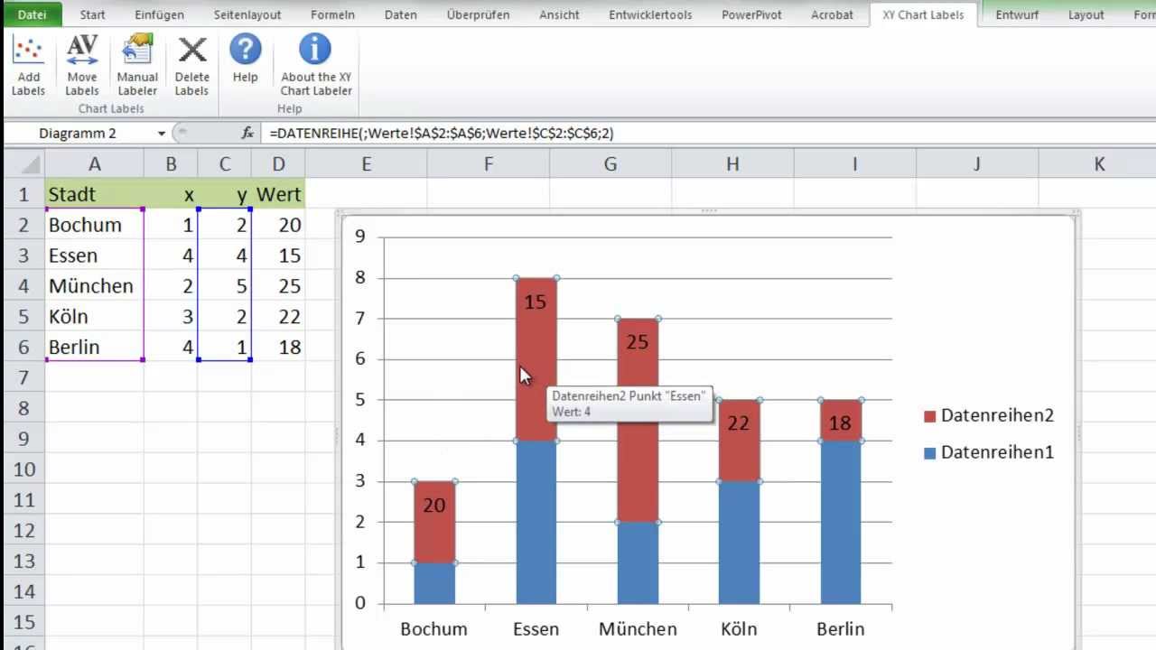
Format Chart Axis in Excel - Axis Options However, In this blog, we will be working with Axis options, Tick marks, Labels, Number > Axis options> Axis options> Format Axis Pane. Axis Options: Axis Options There are multiple options So we will perform one by one. Changing Maximum and Minimum Bounds The first option is to adjust the maximum and minimum bounds for the axis. Two-Level Axis Labels (Microsoft Excel) - ExcelTips (ribbon) Excel automatically recognizes that you have two rows being used for the X-axis labels, and formats the chart correctly. Since the X-axis labels appear beneath the chart data, the order of the label rows is reversed—exactly as mentioned at the first of this tip. (See Figure 1.) Figure 1. Two-level axis labels are created automatically by Excel.

How can I get data labels to show for each column in a bar chart? Turn on 'Overflow text' under Data label' Format tab. Also, you can adjust the position of the Data Label by switching to 'Outside End' or 'Inside Center' so that your Data Label gets displayed properly. If this post helps, then mark it as 'Accept as Solution ' so that it could help others. Regards, Sanket Bhagwat View solution in original post

How to show labels in excel chart

How to Use Excel Pivot Table Label Filters You can use a similar technique to hide most of the items in the Row Labels or Column Labels. Select the pivot table items that you want to keep visible Right-click on one of the selected items In the pop-up menu, click Filter, then click Keep Only Selected Items. All but the selected items are immediately hidden in the pivot table. How to make a scatter plot in Excel - Ablebits Select the Value From Cells box, and then select the range from which you want to pull data labels (B2:B6 in our case). If you'd like to display only the names, clear the X Value and/or Y Value box to remove the numeric values from the labels. Specify the labels position, Above data points in our example. That's it! Text Labels on a Horizontal Bar Chart in Excel - Peltier Tech 21/12/2010 · In this tutorial I’ll show how to use a combination bar-column chart, in which the bars show the survey results and the columns provide the text labels for the horizontal axis. The steps are essentially the same in Excel 2007 and in Excel 2003. I’ll show the charts from Excel 2007, and the different dialogs for both where applicable.

How to show labels in excel chart. How to Find, Highlight, and Label a Data Point in Excel Scatter Plot? By default, the data labels are the y-coordinates. Step 3: Right-click on any of the data labels. A drop-down appears. Click on the Format Data Labels… option. Step 4: Format Data Labels dialogue box appears. Under the Label Options, check the box Value from Cells . Step 5: Data Label Range dialogue-box appears. How to: Display and Format Data Labels - DevExpress To display value labels, set the DataLabelBase.ShowValue property of the DataLabelOptions object to true. Series name. Series labels identify data series to which the data points in the chart belong. Most series include multiple data points, so the same name will be repeated for all data points in the series, which is probably overkill. Custom Axis Labels and Gridlines in an Excel Chart 23/07/2013 · In Excel 2007-2010, go to the Chart Tools > Layout tab > Data Labels > More Data label Options. In Excel 2013, click the “+” icon to the top right of the chart, click the right arrow next to Data Labels, and choose More Options…. Then in all versions, choose the Label Contains option for Y Values and the Label Position option for Left. The labels are (temporarily) shaded … DataLabels.ShowValue property (Excel) | Microsoft Docs Example. This example enables the value to be shown for the data labels of the first series, on the first chart. This example assumes that a chart exists on the active worksheet. VB. Sub UseValue () ActiveSheet.ChartObjects (1).Activate ActiveChart.SeriesCollection (1) _ .DataLabels.ShowValue = True End Sub.

Labeling X-Y Scatter Plots (Microsoft Excel) - ExcelTips (ribbon) Just enter "Age" (including the quotation marks) for the Custom format for the cell. Then format the chart to display the label for X or Y value. When you do this, the X-axis values of the chart will probably all changed to whatever the format name is (i.e., Age). However, after formatting the X-axis to Number (with no digits after the decimal ... How to make a quadrant chart using Excel - Basic Excel Tutorial To create it, follow these steps 1. Click on an empty cell 2. Go to the Insert tab 3. On the Charts dialog box, select the X Y (Scatter) to display all types of charts. 5. Click Scatter. An empty chart will appear on your worksheet. Add values to the chart. 1. Right-click on the empty chart area and choose 'Select Data.' 2. How to Move Excel Pivot Table Labels Quick Tricks Use Menu Commands to Move Label. To move a pivot table label to a different position in the list, you can use commands in the right-click menu: Right-click on the label that you want to move. Click the Move command. Click one of the Move subcommands, such as Move [item name] Up. The existing labels shift down, and the moved label takes its new ... spreadsheeto.com › axis-labelsHow To Add Axis Labels In Excel [Step-By-Step Tutorial] Axis labels make Excel charts easier to understand. Microsoft Excel, a powerful spreadsheet software, allows you to store data, make calculations on it, and create stunning graphs and charts out of your data. And on those charts where axes are used, the only chart elements that are present, by default, include: Axes; Chart Title; Grid lines

Excel Chart Vertical Axis Text Labels • My Online Training Hub Now comes the Sneaky Bar Chart; we know that a bar chart has text labels on the vertical axis like this: ... Layout Tab > Axes > Secondary Vertical Axis > Show default axis. Excel 2013: Chart Tools: Design Tab > Add Chart Element > Axes > Secondary Vertical. Now your chart should look something like this with an axis on every side: Let’s cull some of those axes and format … How to Add a Trendline in Excel Charts | Upwork Let's look at the steps to add a trendline to your chart in Excel. Select the chart Click the Chart Design tab Click Add Chart Element Select Trendline Select the type of trendline In our example, we'll add a trendline to our graph depicting the average monthly temperatures for Texas. How to Add Total Data Labels to the Excel Stacked Bar Chart 03/04/2013 · For stacked bar charts, Excel 2010 allows you to add data labels only to the individual components of the stacked bar chart. The basic chart function does not allow you to add a total data label that accounts for the sum of the individual components. Fortunately, creating these labels manually is a fairly simply process. How to Apply a Filter to a Chart in Microsoft Excel Select the chart and you'll see buttons display to the right. Click the Chart Filters button (funnel icon). When the filter box opens, select the Values tab at the top. You can then expand and filter by Series, Categories, or both. Simply check the options you want to view on the chart, then click "Apply." Advertisement

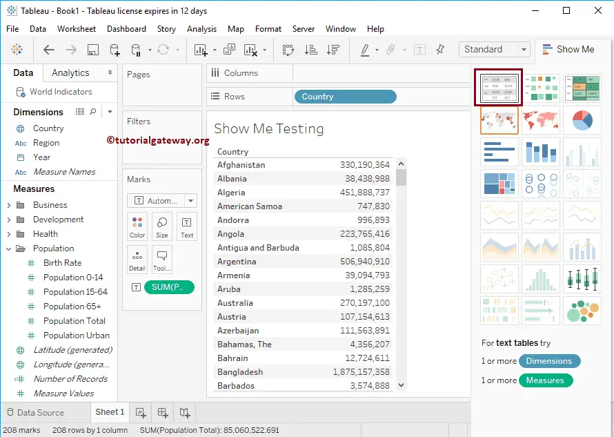
Tableau Show Me

How to Add Labels to Scatterplot Points in Excel - Statology Next, click anywhere on the chart until a green plus (+) sign appears in the top right corner. Then click Data Labels, then click More Options… In the Format Data Labels window that appears on the right of the screen, uncheck the box next to Y Value and check the box next to Value From Cells.

Chart Data Labels in PowerPoint 2011 for Mac

excel - How to not display labels in pie chart that are 0% - Stack Overflow Generate a new column with the following formula: =IF (B2=0,"",A2) Then right click on the labels and choose "Format Data Labels". Check "Value From Cells", choosing the column with the formula and percentage of the Label Options. Under Label Options -> Number -> Category, choose "Custom". Under Format Code, enter the following:

Excel - XY Chart Labeler - Diagramme beschriften - YouTube

How to Change Excel Chart Data Labels to Custom Values? 05/05/2010 · When you “add data labels” to a chart series, excel can show either “category” , “series” or “data point values” as data labels. But what if you want to have a data label that is altogether different, like this: You can change data labels and point them to different cells using this little trick. First add data labels to the chart (Layout Ribbon > Data Labels) Define the …

Excel High Precision Engineering Chart #1 - Excel Hero Blog

Chart.ApplyDataLabels method (Excel) | Microsoft Docs For the Chart and Series objects, True if the series has leader lines. Pass a Boolean value to enable or disable the series name for the data label. Pass a Boolean value to enable or disable the category name for the data label. Pass a Boolean value to enable or disable the value for the data label.

Excel Dashboard Templates Fixing Your Excel Chart When the Multi-Level Category Label Option is ...

Excel Map Chart not showing DATA LABELS for all INDIAN PROVINCES It seems really inconsistent and I would appreciate Micrsoft looking into this. In this following example, this time with India, I'm trying to get my data label (Provinces and data %'s) to appear in white on the map chart, however, they are refusing to appear even though I clicked on all the right areas for them to do so.

34 How To Add Label To Excel Chart

5 New Charts to Visually Display Data in Excel 2019 - dummies Enter the labels and data. Put them in the order you want them to appear in the chart, from top to bottom. You can convert the range to a table to sort it more easily. Select the labels and data and then click Insert → Insert Waterfall, Funnel, Stock, Surface, or Radar Chart → Funnel. Format the chart as desired.

Share :