39 excel chart multi level category labels
Can Excel Map Zip Codes? Map Charts From a Spreadsheet! Excel will give you the map chart based on value or category depending on your data. 4. Customize. Excel arranges the colors by default; however, you can format the map chart in your style using design tools. Open the formatting table by double-clicking on the map chart. You will see the options that you can customize. Chart.CategoryLabelLevel property (Excel) | Microsoft Docs CategoryLabelLevel expression A variable that represents a Chart object. Remarks If there is a hierarchy, 0 refers to the most parent level, 1 refers to its children, and so on. So, 0 equals the first level, 1 equals the second level, 2 equals the third level, and so on. Property value XLCATEGORYLABELLEVEL Example
Excel Waterfall Chart: How to Create One That Doesn't Suck Ideally, you would create a waterfall chart the same way as any other Excel chart: (1) click inside the data table, (2) click in the ribbon on the chart you want to insert. ... in Excel 2016 Microsoft decided to listen to user feedback and introduced 6 highly requested charts in Excel 2016, including a built-in Excel waterfall chart.

Excel chart multi level category labels
Two-Level Axis Labels (Microsoft Excel) - ExcelTips (ribbon) Excel automatically recognizes that you have two rows being used for the X-axis labels, and formats the chart correctly. Since the X-axis labels appear beneath the chart data, the order of the label rows is reversed—exactly as mentioned at the first of this tip. (See Figure 1.) Figure 1. Two-level axis labels are created automatically by Excel. How to Create Organizational Chart in Excel - Computing.NET Step3: Click on the Hierarchy category from the list on the right. Step 4: Select the Organization Chart layout icon from the displayed options on the right. Step 5: Click OK. Step 6: A basic org chart that can be edited is created. To label a position or enter a text into any block, simply click inside the block. Excel Line Column Chart With 2 Axes - Contextures Excel Tips To change a series chart type: In the chart, right-click on one of the selected Cases columns. In the shortcut menu that appears, click Change Series Chart Type In the Change Chart Type dialog box, click on the Line category Next, click on the first Line chart type Click OK to apply the change, and to close the Change Chart Type window.
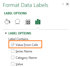
Excel chart multi level category labels. How to Plot Confidence Intervals in Excel (With Examples) A confidence interval represents a range of values that is likely to contain some population parameter with a certain level of confidence.. This tutorial explains how to plot confidence intervals on bar charts in Excel. Example 1: Plot Confidence Intervals on Bar Graph. Suppose we have the following data in Excel that shows the mean of four different categories along with the corresponding ... Per my testing, we may have to manually add it to our data label. The detailed steps are shown in the figure below: But because both Country and Manufacturer columns are category columns, we may not be able to keep only the Country column. Thanks for your understanding. In addition, you can also try to display both in the data bar. Excel Dynamic Chart Linked with a Drop-down List - GeeksforGeeks Follow the below steps to implement a dynamic chart linked with a drop-down menu in Excel: Step 1: Insert the data set into an Excel sheet in the cells as shown above. Step 2: Now select any cell where you want to create the drop-down list for the courses. Step 3: Now click on the Data tab from the top of the Excel window and then click on Data ... How do I format the second level of multi-level category labels ... To set that: Click on the chart Click on the axis label On Format Axis > select Text Options tab > Go to Text box section > Text direction For changing the first level axis label text direction, we would like to invite you share your feedback to Excel · Community (microsoft.com). The Excel team view and take helpful and popular ideas in this way.
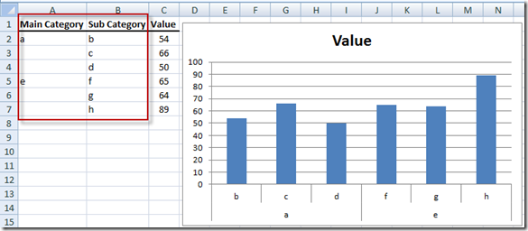
› how-to-create-multiHow to Create Multi-Category Charts in Excel? - GeeksforGeeks May 24, 2021 · The multi-category chart is used when we handle data sets that have the main category followed by a subcategory. For example: “Fruits” is a main category and bananas, apples, grapes are subcategories under fruits. These charts help to infer data when we deal with dynamic categories of data sets. 5 New Charts to Visually Display Data in Excel 2019 - dummies Select the data and labels and then click Insert → Maps → Filled Map. Wait a few seconds for the map to load. Resize and format as desired. For example, you could apply one of the chart styles from the Chart Tools Design tab. To add data labels to the chart, choose Chart Tools Design → Add Chart Element → Data Labels → Show. Types of Graphs - Top 10 Graphs for Your Data You Must Use Add data labels #8 Gauge Chart. The gauge chart is perfect for graphing a single data point and showing where that result fits on a scale from "bad" to "good." Gauges are an advanced type of graph, as Excel doesn't have a standard template for making them. To build one you have to combine a pie and a doughnut. How did I classify 50 chart types by purpose? - Towards Data Science The height of the bar represents the measurement shown on the x-axis. We use the bar chart to display large text labels. A clustered column chart, like a clustered bar chart, is used to compare categories of a categorical variable on some metric. ... Line chart. Multi-series line charts are used to compare how different groups are performing ...
How to Add a Trendline in Excel Charts - Upwork Let's look at the steps to add a trendline to your chart in Excel. Select the chart. Click the Chart Design tab. Click Add Chart Element. Select Trendline. Select the type of trendline. In our example, we'll add a trendline to our graph depicting the average monthly temperatures for Texas. › excel-multi-coloredExcel Multi-colored Line Charts - My Online Training Hub May 08, 2018 · It really depends if you plan to update your chart with new data or not. Option 2: Multi-colored line chart with multiple series. The second option for Excel multi-colored line charts is to use multiple series; one for each color. The chart below contains 3 lines; red, yellow and green. How to Create Charts in Excel: Types & Step by Step Examples Below are the steps to create chart in MS Excel: Open Excel. Enter the data from the sample data table above. Your workbook should now look as follows. To get the desired chart you have to follow the following steps. Select the data you want to represent in graph. Click on INSERT tab from the ribbon. Click on the Column chart drop down button. A Step-By-Step Guide on How to Make a Pie Chart in Excel Select the "Add data labels" option from the drop-down menu when you right-click on the chart to create these titles. Then insert alphabetical or numerical values into the pie chart. You may also select the "Format data labels" and then the "Label options" tab to show or edit the category names.

How to Create Multi-Category Chart in Excel - Excel Board
38 meto price gun labels nz - thedettlingfam.blogspot.com Labels to fit the Meto Eagle 7.22's 1 line of 7 characters Best Before - Meto Price Gun Labels ... - Packaging Products These Meto Labels are pre-printed with "Best Before" and are used with the Meto Date Gun 718. Size: 18mm x 11mm. Pack: 20 Rolls (1500 labels per roll) Black on White Print. Refer Gun Code: LMET0718D. Order Online 24/7.

Nested donut chart (also known as Multi-level doughnut chart, Multi-series doughnut chart ...
› gantt-chart › how-to-makeExcel Gantt Chart Tutorial + Free Template + Export to PPT To create a Gantt chart in Excel that you can use as a template in the future, you need to do the following: List your project data into a table with the following columns: Task description, Start date, End date, Duration. Add a Stacked Bar Chart to your Excel spreadsheet using the Chart menu under the Insert tab.

How to edit the label of a chart in Excel? - Stack Overflow
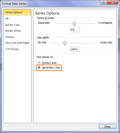
Make Excel charts primary and secondary axis the same scale First create 2 new columns and call then Primary and Secondary Scale. In the first cell create a MIN function that looks at ALL the original data points and finds the smallest number. In the last cell do the same but this time a MAX to find the biggest number out of all the data points. In E8 and E34 just equals to the adjacent cells.

How to Create Multi-Category Chart in Excel - Excel Board
How to Create and Customize a Treemap Chart in Microsoft Excel Either right-click the chart and pick "Format Chart Area" or double-click the chart to open the sidebar. On Windows, you'll see two handy buttons on the right of your chart when you select it. With these, you can add, remove, and reposition Chart Elements. And you can pick a style or color scheme with the Chart Styles button.
Excel Custom Chart Labels • My Online Training Hub
excelfind.com › tutorials › multi-layer-doughnut-chartHow to create a creative multi-layer Doughnut Chart in Excel The core feature of this chart is the gradual multi-layer design, which means a data point has more layers the bigger its value is. At the same time the values are ordered from the biggest to the smallest value which leads to visually appealing flow for the audience’s eyes.
Excel Custom Chart Labels • My Online Training Hub
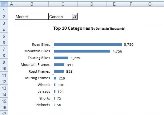
Best Types of Charts in Excel for Data Analysis ... - Optimize Smart #1 Use a bar chart whenever the axis labels are too long to fit in a column chart: What are the different types of bar charts? Horizontal bar charts - Represent the data horizontally. The data categories are shown on the vertical axis, and data values are shown on the horizontal axis. Vertical bar charts - Also called a column chart.

How to Create Multi-Category Chart in Excel - Excel Board
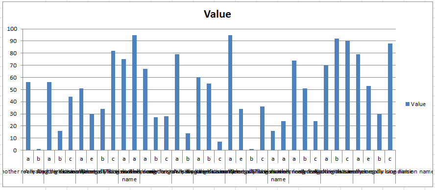
› excel › excel-chartsCreate a multi-level category chart in Excel - ExtendOffice Create a multi-level category column chart in Excel. In this section, I will show a new type of multi-level category column chart for you. As the below screenshot shown, this kind of multi-level category column chart can be more efficient to display both the main category and the subcategory labels at the same time.
Moving X-axis labels at the bottom of the chart below negative values in Excel - PakAccountants.com
How to Use Excel Pivot Table Label Filters To change the Pivot Table option to allow multiple filters: Right-click a cell in the pivot table, and click PivotTable Options. Click the Totals & Filters tab Under Filters, add a check mark to 'Allow multiple filters per field.' Click OK Quick Way to Hide or Show Pivot Items

Create a multi-level category chart in Excel
How to Create a Run Chart in Excel (2021 Guide) | 2 Free Templates Go to the Insert tab. Click " Insert Line or Area Chart .". Choose " Line .". You now have your simple run chart as a result: Step 3. Spruce Up Your Run Chart. Technically, you're good to go, but if you're looking to improve your chart from boring to beautiful in mere moments, here's how you can quickly spruce it up.
Excel Dashboard Templates 3 Ways to Make Excel Chart Horizontal Categories Fit Better - Excel ...
chandoo.org › wp › change-data-labels-in-chartsHow to Change Excel Chart Data Labels to Custom Values? May 05, 2010 · The Chart I have created (type thin line with tick markers) WILL NOT display x axis labels associated with more than 150 rows of data. (Noting 150/4=~ 38 labels initially chart ok, out of 1050/4=~ 263 total months labels in column A.) It does chart all 1050 rows of data values in Y at all times.
How to create an Excel chart with no numerical labels? - Super User
Format Chart Axis in Excel - Axis Options Right-click on the Vertical Axis of this chart and select the "Format Axis" option from the shortcut menu. This will open up the format axis pane at the right of your excel interface. Thereafter, Axis options and Text options are the two sub panes of the format axis pane. Formatting Chart Axis in Excel - Axis Options : Sub Panes
Fixing Your Excel Chart When the Multi-Level Category Label Option is Missing. - Excel Dashboard ...
Two level axis in Excel chart not showing • AuditExcel.co.za You can easily do this by: Right clicking on the horizontal access and choosing Format Axis Choose the Axis options (little column chart symbol) Click on the Labels dropdown Change the 'Specify Interval Unit' to 1 If you want you can make it look neater by ticking the Multi Level Category Labels
34 How To Label A Chart In Excel - Label Ideas 2020
How to Create a Scatterplot with Multiple Series in Excel Step 3: Create the Scatterplot. Next, highlight every value in column B. Then, hold Ctrl and highlight every cell in the range E1:H17. Along the top ribbon, click the Insert tab and then click Insert Scatter (X, Y) within the Charts group to produce the following scatterplot: The (X, Y) coordinates for each group are shown, with each group ...

How to Create Multi-Category Chart in Excel - Excel Board
support.microsoft.com › en-us › officeCreate a Map chart in Excel - support.microsoft.com Just click on the map, then choose from the Chart Design or Format tabs in the ribbon. You can also double-click the chart to launch the Format Object Task Pane, which will appear on the right-hand side of the Excel window. This will also expose the map chart specific Series options (see below).
Formatting Multi-Category Chart Labels | Dashboards & Charts | Excel Forum • My Online Training Hub
How To Show Two Sets of Data on One Graph in Excel To do so, click and drag your mouse across all the data you want, including the names of the columns and rows. You can check that you selected the data by looking for the cells to be gray instead of white. 3. Click the "Insert" tab and then look at the "Recommended Charts" in the charts group

Fixing Your Excel Chart When the Multi-Level Category Label Option is Missing. - Excel Dashboard ...
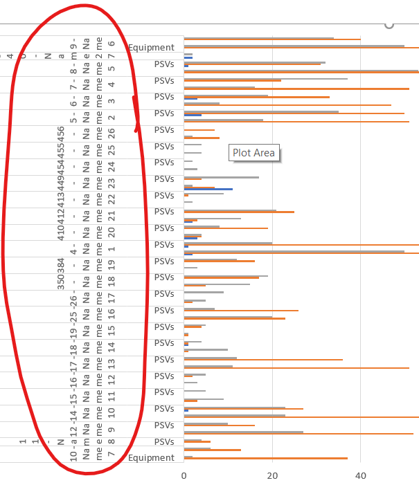
Combination Chart for Multi-Factor Test Results - Peltier Tech The formula in cell F3 (which Excel fills into the whole column of the Table) is =INT ( (ROW ()-ROW ($F$2)+3)/MAX ( [Rep])) Each replicated test takes up a fraction of the width of each category ("Frac" in the table), with the first replication at zero and the last replication at 1. The formula in G3 is = ( [@Rep]-1)/ (MAX ( [Rep])-1)
Post a Comment for "39 excel chart multi level category labels"