40 format data labels pane excel

Edit titles or data labels in a chart - Microsoft Support Reset label text · On a chart, click one time or two times on the data label that you want to link to a corresponding worksheet cell. · Right-click the data label ... Pie of Pie Chart in Excel - Inserting, Customizing - Excel ... This is going to open a Format Data Labels pane at the right of excel. Mark the percentage, category name, and legend key. Select the position of data labels at Outside End. Select the fill color for data labels as white as we will change the chart background in the coming section. You can do it from the fill tab of the opened pane.

How to add data labels from different column in an Excel ... Right click the data series, and select Format Data Labels from the context menu. 3. In the Format Data Labels pane, under Label Options tab, check the Value From Cells option, select the specified column in the popping out dialog, and click the OK button. Now the cell values are added before original data labels in bulk. 4.

Format data labels pane excel

How to format axis labels as thousands/millions in Excel? Right click at the axis you want to format its labels as thousands/millions, select Format Axisin the context menu. 2. In the Format Axisdialog/pane, click Number tab, then in theCategorylist box, select Custom, and type[>999999] #,,"M";#,"K"into Format Codetext box, and click Addbutton to add it toTypelist. See screenshot: 3. How do you format data series in Excel? To format data labels in EÎl , choose the set of data labels to format . To do this, click the " Format " tab within the "Chart Tools" contextual tab in the Ribbon. Then select the data labels to format from the "Chart Elements" drop-down in the "Current Selection" button group. How do I show the Format Data Series pane in Excel? How to stagger axis labels in Excel In the chart, righ-click the "+ labels" data series and select Add Data Labels from the shortcut menu. 15. Next, right-click the Series "+ label" Data Labels and then, on the shortcut menu, click Format Data Labels. 16. In the Format Data Labels pane, with Label Options selected, set the Label Position to Below. 17.

Format data labels pane excel. Format Data Labels in Excel- Instructions - TeachUcomp, Inc. To format data labels in Excel, choose the set of data labels to format. To do this, click the "Format" tab within the "Chart Tools" contextual tab in the Ribbon. Then select the data labels to format from the "Chart Elements" drop-down in the "Current Selection" button group. How to Print Labels From Excel? | Steps to Print Labels ... Navigate towards the folder where the excel file is stored in the Select Data Source pop-up window. Select the file in which the labels are stored and click Open. A new pop up box named Confirm Data Source will appear. Click on OK to let the system know that you want to use the data source. Again a pop-up window named Select Table will appear. Pie Chart in Excel - Inserting, Formatting, Filters, Data ... Right click on the Data Labels on the chart. Click on Format Data Labels option. Consequently, this will open up the Format Data Labels pane on the right of the excel worksheet. Mark the Category Name, Percentage and Legend Key. Also mark the labels position at Outside End. This is how the chark looks. Formatting the Chart Background, Chart Styles Format elements of a chart - Microsoft Support Change format of chart elements by using the Format task pane or the ribbon. You can format the chart area, plot area, data series axes, titles, data labels ...

Excel tutorial: How to use data labels When first enabled, data labels will show only values, but the Label Options area in the format task pane offers many other settings. You can set data labels to show the category name, the series name, and even values from cells. In this case for example, I can display comments from column E using the "value from cells" option. Using Graphics to Represent Data Series (Microsoft Excel) Choose Format Data Series from the Context menu. Excel displays the Format Data Series task pane at the right side of the chart. In the task pane click the Fill & Line icon; it looks like a spilling paint bucket. Expand the Fill options by clicking the small triangle next to the Fill heading. (See Figure 2.) Figure 2. The Fill options of the ... Adding rich data labels to charts in Excel 2013 ... In the Formatting Task Pane, you can customize the way the data labels appear, change their size and alignment, change their text properties, and even add another data series for them to include. See Format and customize Excel 2013 charts quickly with the new Formatting Task pane for more discussion about the Formatting Task Pane in general. Add a DATA LABEL to ONE POINT on a ... - Excel Quick Help You can now configure the label as required — select the content of the label (e.g. series name, category name, value, leader line), the position (right, left, above, below) in the Format Data Label pane/dialog box. To format the font, color and size of the label, now right-click on the label and select 'Font'. Note: in step 5. above, if ...

Excel Charts - Aesthetic Data Labels - Tutorialspoint To format the data labels − Step 1 − Right-click a data label and then click Format Data Label. The Format Pane - Format Data Label appears. Step 2 − Click the Fill & Line icon. The options for Fill and Line appear below it. Step 3 − Under FILL, Click Solid Fill and choose the color. PDF Where is the format data labels task pane in excel In the Format Data Labels pane: On the Label Options tab: In the Label Contains group, select Value, In the Label Position group, select Inside Base: On the Number tab, in the Category list, select Custom, enter format that you want in the Format Code field and press Add: For more details, see Conditional formatting of chart axes. How to Print Labels from Excel - Lifewire Select Mailings > Write & Insert Fields > Update Labels . Once you have the Excel spreadsheet and the Word document set up, you can merge the information and print your labels. Click Finish & Merge in the Finish group on the Mailings tab. Click Edit Individual Documents to preview how your printed labels will appear. Select All > OK . How to Customize Your Excel Pivot Chart Data Labels - dummies Excel displays the Format Data Labels pane. Check the box that corresponds to the bit of pivot table or Excel table information that you want to use as the label. For example, if you want to label data markers with a pivot table chart using data series names, select the Series Name check box.

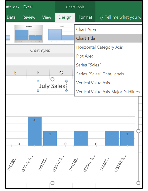
Excel 2016 charts: How to use the new Pareto, Histogram, and Waterfall formats | PCWorld

2/ Right-click i.e. on the 1st histo. bar (A) > Add Data Labels (numbers are displayed a the top of the bars) 3/ Click one of the numbers that just displayed (the Format Data Labels pane opens on the right) > Check option "Value From Cells" > Select range C2:C7 > OK > Uncheck option "Value" demo.png (18.5 KiB) · 3

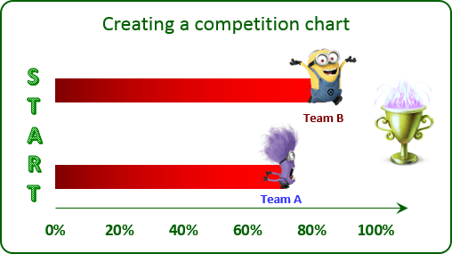
Creating a simple competition chart - Microsoft Excel 2013

Format Data Labels Task Pane Excel How To Format Data Labels In Excel - Walls Alawavell Details: Step 1 − Click on the Data Label, whose Fill colour you want to change. Double click to change the Fill color for only one Data Characterization. The Format Information Characterization Task Pane appears. Step 2 − Click Fill → Solid Fill.

How to make a histogram in Excel 2019, 2016, 2013 and 2010

Formatting Data Labels Ribbon: On the Series tab, in the Properties group, open the Data Labels drop-down menu and select More Data Labels Options to open the Format Labels dialog box ...

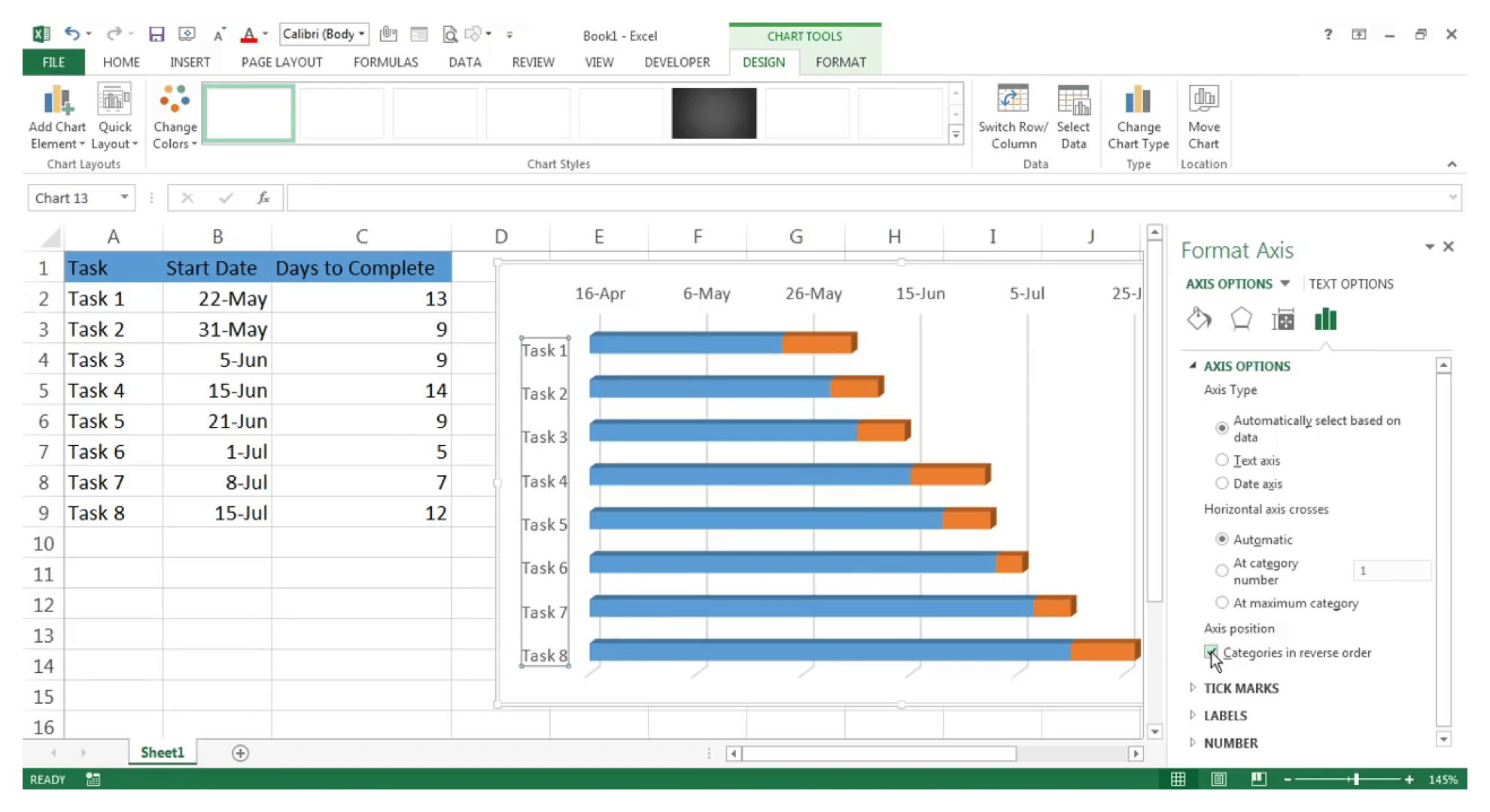
How to Make Gantt Chart in Excel? | Gantt Chart Excel - Zoho Projects

Add or remove data labels in a chart - Microsoft Support Right-click the data series or data label to display more data for, and then click Format Data Labels. Click Label Options and under Label Contains, select the Values From Cells checkbox. When the Data Label Range dialog box appears, go back to the spreadsheet and select the range for which you want the cell values to display as data labels.

Share :